Block Execution Order, Feedback Loops, and Statefulness

Converting a control flow diagram into a sequence of discretely executed functions in code is challenging. Though the execution order may seem obvious visually, establishing the correct semantics programmatically—especially in large, complex models—is far from trivial.

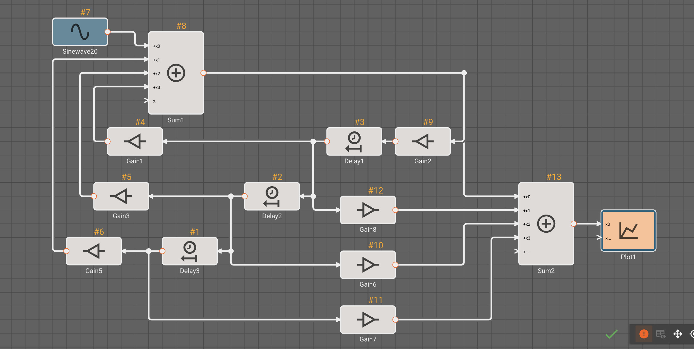Block execution order of a nested feedback loop. Numbers in orange above each block indicate their execution order in generated code.

The primary principle governing block execution order is data dependency. A block cannot compute its output until all the blocks providing its input signals have already executed in the current simulation step. For simple feed-forward paths, where signals flow in a single direction, this naturally leads to an execution order progressing from input sources toward output sinks.

The Challenge of Feedback Loops

Complexity increases dramatically with feedback loops, also known as graph cycles. A feedback loop exists when tracing a block's input dependencies eventually leads back to that same block’s output. This creates a circular dependency where Block A requires Block B’s output, but Block B simultaneously requires Block A’s output within the same simulation step.

Resolving these circular dependencies requires “grounding” the loop with a block whose output can be determined independently of its inputs in the current time step. These are referred to as stateful blocks.

Stateful Blocks as Loop Resolvers

Stateful blocks are characterized by maintaining an internal state that persists between simulation steps. This state allows them to provide a valid output at the beginning of a simulation step before their inputs for that step have been fully computed.

Consider a simple integrator: We often want to set the Initial Condition of the integrator, so that it starts with a pre-determined output value before any computation has occurred. This makes an integrator an excellent candidate for feedback loop resolution. Its initial condition can be used by the blocks which depend on it, and then their outputs can be used to update the integrator.

For the first simulation step (t = 0), the output of a stateful block is determined by its configured Initial Condition. For all subsequent steps (t > 0), its output at the start of the step is the value its state held at the end of the previous time step (t - 1). Because this output value is available upfront, the computation within the loop can begin, effectively “breaking” the circular dependency for the current step.

Stateful vs. Stateless Blocks

All blocks can be categorized as either stateful or stateless:

• A stateless block is one whose output is determined entirely by its current inputs and carries no internal state that influences the computation across time steps. A trigonometric function like cosine(x) is a prime example; its output depends only on the current input x.
• A stateful block, conversely, stores state between execution steps (e.g., the current value of an integration or the previous input value), and its output depends on both current inputs and its internal state.

Stateful blocks are crucial for enabling the execution of feedback loops. If Pictorus detects a cyclical feedback loop in your model that does not contain at least one stateful block to provide a starting point, an error will be raised identifying the blocks involved and indicating the need to insert a stateful element to resolve the dependency.

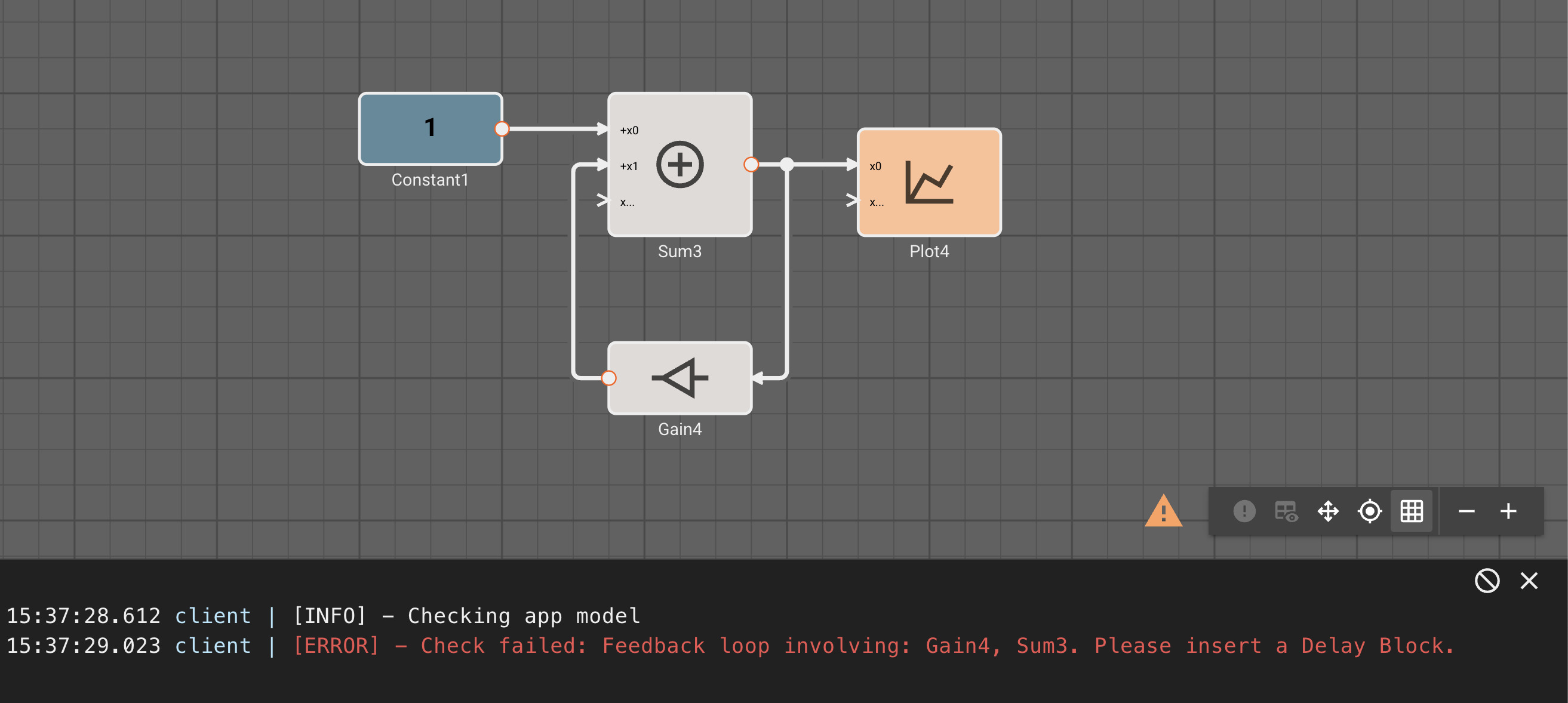Errors tell you exactly which blocks are involved in a feedback loop and must be resolved with a stateful block.

The Role of Delay Blocks

Delay blocks, particularly unit delays (delays of exactly one timestep), are a convenient and idiomatic choice for resolving feedback loops when no other stateful block naturally exists within the cycle. A unit delay block introduces minimal computational complexity other than shifting the signal in time. Since stateful blocks are prioritized for early execution within a loop, the delay block’s output at the start of the step is simply the value from the loop in the previous iteration. On the first iteration, its output is its initial condition. This behavior provides the necessary causal break without altering the fundamental dynamics of the loop, making it the standard tool for loop resolution.

Handling Complex and Nested Loops

As illustrated in the title graphic, complex models often feature nested feedback loops and intertwined feed-forward paths. Pictorus employs a sophisticated algorithm that analyzes all signal paths, identifies dependencies, and locates stateful blocks to determine a valid, causally correct execution order for the entire model.

While the algorithm ensures that feedback loops are resolvable using stateful blocks, the presence of multiple stateful blocks within a single loop introduces additional considerations. The solver must still determine an execution order that respects dependencies between the stateful elements themselves. Improper placement of multiple stateful blocks can inadvertently introduce unintended delays into the feedback path, potentially leading to unexpected or undesirable system behavior.

Pictorus takes care to minimize solver-induced delays, prioritizing an order that relies on the user’s explicit stateful elements. However, understanding the determined execution order is key for debugging. If certain portions of your control diagram exhibit odd output behavior, it is possible that the arrangement of stateful blocks is causing unintended delays. Use the "Show Issues" feature in the UI to manually inspect detected loops and the calculated block execution order within them, helping you identify placements that could be rewritten to better align with your intended system dynamics.